|
Size: 37
Comment:
|
Size: 20035
Comment:
|
| Deletions are marked like this. | Additions are marked like this. |
| Line 2: | Line 2: |
| The {{attachment:search_perspective.png}} perspective provides the following search types: * Dependency-Search * * Coreference-Documents * * !ErrorMining for Part-Of-Speech Tags * * !ErrorMining for Dependency Structure . * under development will be available soon ===== How to set up a new search: ===== 1. Click on {{attachment:search_new.png}} to create a new search. 1. Afterwards the search need to be configured: 1. {{attachment:search_configuration.png||align="top"}} * Type: Select one of the following search types described above. * Data-Set: The Treebank/Document used for the query. * Query: Clicking {{attachment:search_query.png}} opens the query editor. There may be different types of query editors depending on the search type. * Parameters: Search pararameters depending on the search type. 1. Execute Search using the {{attachment:search_execute.png}} button 1. View the Result by double-clicking the search result or use the inspect-button {{attachment:search_inspect.png}} ===== Search Parameters (Dependency-Search): ===== * Search-Mode: Non-Exhaustive (stop after first hit), Exhaustive (add each sentence to the result at most one) and Exhaustive search with Grouping * Direction: Left-To-Right or Right-To-Left * Case-Sensitiv: On/Off * Result Limit: limit the search result (number of hits) ===== Result Outline(Dependency-Search): ===== [[attachment:search_result_1D.png|{{attachment:search_result_1D.png|attachment:search_result_1D.png|width="400"}}]] * Aggregated result visualization depending on the number of grouping operators (dimensions) for up to three groups (3D) * Result highlighting for instances of query constraints * Fully customizable graph visualization * Easy navigation through results for up to three groups (3D) ==== Search Menu: ==== {{attachment:search_manager_menu.png}} * {{attachment:search_preferences.png}} = Open the preferences * {{attachment:search_new.png}} = Create a new search * {{attachment:search_execute.png}} = Executes the search. Note if no data-set was set the button is disabled {{attachment:search_execute_inactive.png}} Search History Toolbar: {{attachment:search_history-tb.png}} . Every executed search is listed in the search history. The history is available until you close your ICARUS session. The figure shows three search history items. During the search process the icons to the left may change: * {{attachment:search_runing+loading.png|search_runing+loading.png}} Search is active (first icon) but the target data-set is not loaded yet (second icon) * {{attachment:search_runing+loaded.png|search_runing+loaded.png}} Search is active (first icon) and target data-set is loaded (second icon) * {{attachment:search_finished+loaded.png|search_finished+loaded.png}} Search finished successful (first icon) and target data-set is loaded (second icon) * {{attachment:search_icon_error.png}} Search was not successful. * {{attachment:search_clearhistory.png}} = Clear all search history items * {{attachment:search_remove1search.png}} = Remove the selected search result from the history * {{attachment:search_viewquery.png}} = Display the query of the selected search * {{attachment:search_inspect.png}} = Display the result of selected search * {{attachment:search_cancel.png}} Cancel selected search ==== Graph Query Editor: ==== {{attachment:search_query-editor-tab.png}} This tab is used to build a query. Graph Editor Toolbar: {{attachment:search_graph-tb.png}} * {{attachment:search_preferences.png}} = Open the preferences * {{attachment:search_arc-layout.png}} = Change the current graph layout. There are three different layout types available {{attachment:search_qe_layouts.png||align="middle"}} 1. Arc layout {{attachment:search_qe_arc-layout.png||align="middle"}} 1. No layout {{attachment:search_qe_no-layout.png||align="middle"}} 1. Tree {{attachment:search_qe_tree-layout.png||align="middle"}} * {{attachment:search_clear.png}} = Clear graph panel - every nodes/edges are deleted * {{attachment:search_export.png}} = Save the current search graph to XML file (may be imported later) * {{attachment:search_import.png}} = Import a search graph XML file * {{attachment:search_print.png}} = Print the current graph * {{attachment:search_add-node.png}} = Add a new node to the current search graph * {{attachment:search_add-disjunction.png}} = Adds a new disjunction to the current search graph * {{attachment:search_add-edge.png}} = Connects two nodes (two nodes must be selected before this action can be performed) * {{attachment:search_add-pedge.png}} = Connects two nodes with a precedence relation (two nodes must be selected before this action can be performed) * {{attachment:search_delete.png}} = Delete selected node/edge (multi selection possible) * {{attachment:search_edit.png}} = Opens the edit node/edge dialog (Instead of using this button you may doubleclick a node/edge to open the edit dialog) * {{attachment:search_clone.png}} = Duplicate (copy and insert) the selected nodes/edges. Quick way to duplicate a graph. Note: edges are only copied when their source and target node is selected. * {{attachment:search_copy_button.png}} = Copy and the selected nodes/edges. Note: edges are only copied when their source and target node is selected. (strg+c) * {{attachment:search_paste_button.png}} = Paste previously copied nodes/edges. (strg+p) * {{attachment:search_reorder-graph.png}} = Redraw the graph, can be useful while adding new nodes, edges or constraints may mess up the graph layout. Example (arc-layout): (left nodes/edges unsorted; right nodes/edges reorderes) {{attachment:search_graph-redraw.png||align="middle"}} Note: The copy&paste nodes/edges can be used to copy graphs from/into other perspectives (e.g. Tutorial 1D,..) * {{attachment:search_undo.png}} = Undo the last graph editor operation * {{attachment:search_redo.png}} = Redo the last graph editor operation * {{attachment:search_zin.png}} = Increase zoom level * {{attachment:search_zdefault.png}} = Switch back to the default zoom level * {{attachment:search_zout.png}} = Decrease zoom level * {{attachment:search_zauto.png}} = Autofit zoom level to the current graph panel size (default off) * {{attachment:search_zcompress.png}} = Compress graph (right-left). Merge node/edge information into a node. Search annotation highlight is never merged and always visible even. (default off) * {{attachment:search_toggle_c-d.png}} = If there are different (unconnected) graphs A, B the search will use the following query (A v B). Text Query Editor Toolbar: {{attachment:search_query-tb-text.png}} * {{attachment:search_undo.png}} = Undo the last text editor operation * {{attachment:search_redo.png}} = Redo the last text editor operation * {{attachment:search_copy_button.png}} = Copy and the selected text. (strg+c) * {{attachment:search_paste_button.png}} = Paste previously copied text. (strg+p) * {{attachment:search_select-all.png}} = Select the entire query text (strg+a) * {{attachment:search_clearhistory.png}} = Clear the text query panel. * {{attachment:search_save-graph-to-desc.png}} = Save query graph to the current selected search history item * {{attachment:search_sync-to-graph.png}} = Generate search graph from text query * {{attachment:search_sync-to-text.png}} = Generate text query from search graph ==== Result Outline: ==== {{attachment:search_result-tab.png}} Use this tab to browse the search results. The visialization may be seperated into four differnet presentation styles. We describe the different types in the following section. Toolbar {{attachment:search_result-base-tb.png}} * {{attachment:search_preferences.png}} = Open the preferences * {{attachment:search_result-search-desc.png}} Short query description and number of matches (here 3 grouping operators and 10 matches) * {{attachment:search_reorder-graph.png}} = Refresh the result outline * {{attachment:search_export.png}} = Save the current search result to a XML file (may be imported later) * {{attachment:search_import.png}} = Import search result XML file * {{attachment:search_clearhistory.png}} = Close the result outline * {{attachment:search_result-grouping-desc.png}} Grouping operator {{attachment:search_grouping-operator.png}} result informations. The corresponding {{attachment:search_grouping-operator.png}} color and the number of matches for each {{attachment:search_grouping-operator.png}} (ICARUS supports up to three grouping operators) (In this example we have 1. lemma-{{attachment:search_grouping-operator.png}} (red) 8 matches, 2. lemma-{{attachment:search_grouping-operator.png}} (green) 5 matches and 3. pos-{{attachment:search_grouping-operator.png}} 4 matches) 0. No grouping operator {{attachment:search_grouping-operator.png}} is used. * Query: {{attachment:search_query-0D.png||align="middle"}} * Text Query: [lemma=be [relation=VC, pos=VBN]] * Result Toolbar: {{attachment:search_result-tb-0D.png}} The result is presented as a list of sentences. Every occurence that matches the query is colored blue. Results (0D) [[attachment:search_result_0D.png|{{attachment:search_result_0D.png|attachment:search_result_0D.png|width="300"}}]] 1. One grouping operator {{attachment:search_grouping-operator.png}} used. * Query: {{attachment:search_query-1D.png||align="middle"}} * Text Query: [lemma=be [relation=VC, lemma<*>1, pos=VBN]] * Result Toolbar: {{attachment:search_result-tb-1D.png}} All lemma types found are shown in the list (red) to the left. The user may select one lemma type to get all instances with matching query. Every occurence that matches the query is colored blue and the "grouped" lemma colored red. Results (1D) [[attachment:search_result_1D.png|{{attachment:search_result_1D.png|attachment:search_result_1D.png|width="300"}}]] * Options: {{attachment:search_result-option-1D.png}} * {{attachment:search_numeric_switch.png}} = Switch between numeric/percentage result numbers (total) * {{attachment:search_sort.png}} = Sort by wordform or by occurence (ascending/descending) * {{attachment:search_reset_sort.png}} = Reset list sorting 2. Two grouping operator {{attachment:search_grouping-operator.png}} used. * Query: {{attachment:search_query-2D.png||align="middle"}} * Text Query: [lemma=be [relation=VC, lemma<*>1, pos=VBN [relation=LGS, form=by [relation=PMOD, lemma<*>2]]]] * Result Toolbar: {{attachment:search_result-tb-2D.png}} The result is presented as a table. Grouping operator one (red) is on the y-axis and grouping operator two (green) on the x-axis (Note: The x-/y-axis may be fliped clicking on {{attachment:search_flip-table.png}}). Every occurence that matches the query is colored blue. Results (2D) [[attachment:search_result_2D-a.png|{{attachment:search_result_2D-a.png|attachment:search_result_2D-a.png|width="300"}}]] [[attachment:search_result_2D-b.png|{{attachment:search_result_2D-b.png|attachment:search_result_2D-b.png|width="300"}}]] * Options: {{attachment:search_result-option-2D.png}} * {{attachment:search_numeric_switch.png}} = Switch between numeric/percentage result numbers (total) * {{attachment:search_sort.png}} = Sort y-axis by wordform or by occurence (ascending/descending) * {{attachment:search_sort_x-axis.png}} = Sort x-axis by wordform or by occurence (ascending/descending) * {{attachment:search_flip-table.png}} = Swap the x-/y-axis (e.g.: (old) x-axis = (new) y-axis and vice versa) * {{attachment:search_reset_sort.png}} = Reset table sorting 3. Two grouping operator {{attachment:search_grouping-operator.png}} used. * Query: {{attachment:search_query-3D.png||align="middle"}} * Text Query: [lemma=be [relation=VC, lemma<*>1, pos=VBN [relation=LGS, form=by [relation=PMOD, lemma<*>2]][relation=OBJ, lemma<*>3]]] * Result Toolbar: {{attachment:search_result-tb-3D.png}} The result is presented as a list of sentences. Every occurence that matches the query is colored blue. Results (3D) [[attachment:search_result_3D-a.png|{{attachment:search_result_3D-a.png|attachment:search_result_3D-a.png|height="170"}}]] [[attachment:search_result_3D-b.png|{{attachment:search_result_3D-b.png|attachment:search_result_3D-b.png|width="300"}}]] * Options: {{attachment:search_result-option-3D.png}} * {{attachment:search_numeric_switch.png}} = Switch between numeric/percentage result numbers (total) * {{attachment:search_sort.png}} = Sort by wordform or by occurence (ascending/descending) * {{attachment:search_reset_sort.png}} = Reset list sorting * {{attachment:search_sort.png}} = Sort y-axis by wordform or by occurence (ascending/descending) * {{attachment:search_sort_x-axis.png}} = Sort x-axis by wordform or by occurence (ascending/descending) * {{attachment:search_flip-table.png}} = Swap the x-/y-axis (e.g.: (old) x-axis = (new) y-axis and vice versa) * {{attachment:search_reset_sort.png}} = Reset table sorting * {{attachment:search_3D-reorder.png}} = Change the grouping operor ([0] = list, [1] = table y-axis and [2] = table x-axis). In this example {{attachment:search_3D-reorder-dialog.png||align="middle"}} we have [0] = first {{attachment:search_grouping-operator.png}} (red), [1] = second {{attachment:search_grouping-operator.png}} (green) and [3] = third {{attachment:search_grouping-operator.png}} (brown) ===== 1) Tutorial Dependency Search (passive constructions) with one grouping operator: ===== If the the user doesn't exactly know the how passive constructions are annotated in a treebank. Then he can use e.g. mate-tools or weblicht to parse a sentence contains a passice construction and copy&paste the structure to the search graph. 1. Parsed sentence "Mary was kissed by a boy." {{attachment:search_example_mt.png}} . 1. Select the passice construction {{attachment:search_example_mt_selected.png}} 1. Copy the selected cells and edges {{attachment:search_copy.png}} and switch to the {{attachment:search_perspective.png}} 1. Paste selected cells and edges into the search query editor window {{attachment:search_paste.png}} 1. The resulting graph when using the arc-layout (recommended) {{attachment:search_arc-layout.png}} {{attachment:search_cp-graph-arc.png}} 1. In the following step the search graph (query) will be generalized (double clicking the edge / nodes to open the edge/node editor). 1. Node 1 properties {{attachment:search_edit-node.png}} changed to {{attachment:search_edit-node-b.png}} 1. Edge properties {{attachment:search_example-edge.png}} changed to {{attachment:search_example-edge-b.png}} 1. Node 2 properties {{attachment:search_example-node2.png}} changed to (added grouping operator <*>) {{attachment:search_example-node2-b.png}} {{attachment:search_example-node2-c.png}} 1. These changes result in a new more generalized version of the search graph (below is the textual query representation) {{attachment:search_example_sg+text.png|search_example_sg+text.png}} This query matches passive constructions in English as annotated in the CoNLL08 Shared Task data set. 1. Results (1D) [[attachment:search_result_1D.png|{{attachment:search_result_1D.png|attachment:search_result_1D.png|width="400"}}]] ===== 2) Tutorial Dependency Search (passive constructions with overt logical subjects): ===== We are interested in passive constructions with overt logical subjects, grouped by lemma of the verb and the lemma of the logical subject. We may use the search graph for passive constructions or build the query completly manually (shown here). 1. First of all clear the graph editor panel (if there is any remaining graph) using {{attachment:search_clear.png}} 1. Add four new nodes {{attachment:search_add-node.png}} you may "automatic reorder" them by clicking {{attachment:search_reorder-graph.png}} 1. Your graph editor should look like {{attachment:search_t2_4nodes.png}} 1. There are two ways connecting nodes / adding edges 1. Select two nodes {{attachment:search_t2_addingedge-a.png}} and connect them clicking on {{attachment:search_add-edge.png}} 1. Place the cursor in the middle of the desired (source) node. A green border will show up {{attachment:search_hl-node.png}} . Hold the left mousebutton and move to the (target) node. When you reached the target node again a green border shows up. Release the left mousebutton to draw an edge between those node {{attachment:search_t2_addingedge-b.png}} 1. Double click on the nodes/edges to specify the constraints. (Note: Adding constraints may mess up the graph layout. You may use {{attachment:search_reorder-graph.png}} to redraw the graph) 1. Node 1: Lemma = be {{attachment:search_t2-n1.png}} 1. Node 2: Lemma = <*> (red grouping operator); Part-Of-Speech = VBN {{attachment:search_t2-n2.png}} 1. Node 3: Form = by {{attachment:search_t2-n3.png}} 1. Node 4: Lemma = <*> (green grouping operator) {{attachment:search_t2-n4.png}} 1. Edge 1: Relation = VC {{attachment:search_t2-e1.png}} 1. Edge 2: Relation = LGS {{attachment:search_t2-e2.png}} 1. Edge 3: Relation = PMOD {{attachment:search_t2-e3.png}} 1. When every node, edge was linked and there was no error setting the constraints above the search graph should look like this: {{attachment:search_t2-sg.png}} . (Textual query: [lemma=be [relation=VC, lemma<*>1, pos=VBN [relation=LGS, form=by [relation=PMOD, lemma<*>2]]]]) 1. Results (2D) [[attachment:search_result_2D-a.png|{{attachment:search_result_2D-a.png|attachment:search_result_2D-a.png|width="400"}}]] [[attachment:search_result_2D-b.png|{{attachment:search_result_2D-b.png|attachment:search_result_2D-b.png|width="400"}}]] ===== 3) Tutorial Dependency Search (passive constructions with overt logical subjects and object): ===== In tutorial 1) we showed how to create a query using a copied graph from the parser. Tutorial 2) shows how to create a query from scratch. In tutorial 3) we will extend the search graph used in 2) with an additional grouping operator. 1. We start with the following search graph {{attachment:search_t2-sg.png}} 1. Add one new node {{attachment:search_add-node.png}} you may "automatic reorder" them by clicking {{attachment:search_reorder-graph.png}} 1. Your graph editor should look like {{attachment:search_t3-n5added.png}} 1. Connect the "red" node with the new node using one of the following options 1. Select the node {{attachment:search_t3-addedge-c.png}} and connect them clicking on {{attachment:search_add-edge.png}} 1. Place the cursor in the middle of node 2. A green border will show up {{attachment:search_t3-addedge-a.png}} . Hold the left mousebutton and move to the new node. When you reached the target node again a green border shows up {{attachment:search_hl-node.png}} . Release the left mousebutton to draw an edge between those node {{attachment:search_t3-addedge-b.png}} 1. Double click on the new node/edge to specify the constraints. (Note: Adding constraints may mess up the graph layout. You may use {{attachment:search_reorder-graph.png}} to redraw the graph) 1. Node 5: Lemma = <*> (browngrouping operator) {{attachment:search_t3-n5.png}} 1. Edge 4: Relation = OBJ {{attachment:search_t3-e4.png}} 1. When every node, edge was linked and there was no error setting the constraints above the search graph should look like this: {{attachment:search_t3-sg.png}} . (Textual query: [lemma=be [relation=VC, lemma<*>1, pos=VBN [relation=LGS, form=by [relation=PMOD, lemma<*>2]][relation=OBJ, lemma<*>3]]]) 1. Results (3D) [[attachment:search_result_3D-a.png|{{attachment:search_result_3D-a.png|attachment:search_result_3D-a.png|height="170"}}]] [[attachment:search_result_3D-b.png|{{attachment:search_result_3D-b.png|attachment:search_result_3D-b.png|width="400"}}]] |
ICARUS-Search-Perspective
The  perspective provides the following search types:
- Dependency-Search
- * Coreference-Documents
* ErrorMining for Part-Of-Speech Tags
* ErrorMining for Dependency Structure
- * under development will be available soon
How to set up a new search:
Click on
 to create a new search.
 - Afterwards the search need to be configured:

- Type: Select one of the following search types described above.
- Data-Set: The Treebank/Document used for the query.
Query: Clicking
 opens the query editor. There may be different types of query editors depending on the search type.
 - Parameters: Search pararameters depending on the search type.
Execute Search using the
 button
 View the Result by double-clicking the search result or use the inspect-button

Search Parameters (Dependency-Search):
- Search-Mode: Non-Exhaustive (stop after first hit), Exhaustive (add each sentence to the result at most one) and Exhaustive search with Grouping
- Direction: Left-To-Right or Right-To-Left
- Case-Sensitiv: On/Off
- Result Limit: limit the search result (number of hits)
Result Outline(Dependency-Search):
- Aggregated result visualization depending on the number of grouping operators (dimensions) for up to three groups (3D)
- Result highlighting for instances of query constraints
- Fully customizable graph visualization
- Easy navigation through results for up to three groups (3D)
Search Menu:

 = Open the preferences
  = Create a new search
  = Executes the search. Note if no data-set was set the button is disabled
Search History Toolbar:  . Every executed search is listed in the search history. The history is available until you close your ICARUS session. The figure shows three search history items. During the search process the icons to the left may change:
 Search is active (first icon) but the target data-set is not loaded yet (second icon)
  Search is active (first icon) and target data-set is loaded (second icon)
  Search finished successful (first icon) and target data-set is loaded (second icon)
  Search was not successful.
  = Clear all search history items
  = Remove the selected search result from the history
  = Display the query of the selected search
  = Display the result of selected search
  Cancel selected search
Graph Query Editor:
 This tab is used to build a query. Graph Editor Toolbar:
 = Open the preferences
  = Change the current graph layout. There are three different layout types available
Arc layout

No layout

Tree
 = Clear graph panel - every nodes/edges are deleted
  = Save the current search graph to XML file (may be imported later)
  = Import a search graph XML file
  = Print the current graph
  = Add a new node to the current search graph
  = Adds a new disjunction to the current search graph
  = Connects two nodes (two nodes must be selected before this action can be performed)
  = Connects two nodes with a precedence relation (two nodes must be selected before this action can be performed)
  = Delete selected node/edge (multi selection possible)
  = Opens the edit node/edge dialog (Instead of using this button you may doubleclick a node/edge to open the edit dialog)
  = Duplicate (copy and insert) the selected nodes/edges. Quick way to duplicate a graph. Note: edges are only copied when their source and target node is selected.
  = Copy and the selected nodes/edges. Note: edges are only copied when their source and target node is selected. (strg+c)
  = Paste previously copied nodes/edges. (strg+p)
  = Redraw the graph, can be useful while adding new nodes, edges or constraints may mess up the graph layout. Example (arc-layout): (left nodes/edges unsorted; right nodes/edges reorderes)
Note: The copy&paste nodes/edges can be used to copy graphs from/into other perspectives (e.g. Tutorial 1D,..)
 = Undo the last graph editor operation
  = Redo the last graph editor operation
  = Increase zoom level
  = Switch back to the default zoom level
  = Decrease zoom level
  = Autofit zoom level to the current graph panel size (default off)
  = Compress graph (right-left). Merge node/edge information into a node. Search annotation highlight is never merged and always visible even. (default off)
  = If there are different (unconnected) graphs A, B the search will use the following query (A v B).
Text Query Editor Toolbar: 
 = Undo the last text editor operation
  = Redo the last text editor operation
  = Copy and the selected text. (strg+c)
  = Paste previously copied text. (strg+p)
  = Select the entire query text (strg+a)
  = Clear the text query panel.
  = Save query graph to the current selected search history item
  = Generate search graph from text query
  = Generate text query from search graph
Result Outline:
 Use this tab to browse the search results. The visialization may be seperated into four differnet presentation styles. We describe the different types in the following section.
Toolbar 
 = Open the preferences
  Short query description and number of matches (here 3 grouping operators and 10 matches)
  = Refresh the result outline
  = Save the current search result to a XML file (may be imported later)
  = Import search result XML file
  = Close the result outline
  Grouping operator
  result informations. The corresponding
  color and the number of matches for each
  (ICARUS supports up to three grouping operators) (In this example we have 1. lemma-
 (red) 8 matches, 2. lemma-
 (green) 5 matches and 3. pos-
 4 matches)
0. No grouping operator  is used.
Query:

- Text Query: [lemma=be [relation=VC, pos=VBN]]
Result Toolbar:

The result is presented as a list of sentences. Every occurence that matches the query is colored blue. Results (0D) 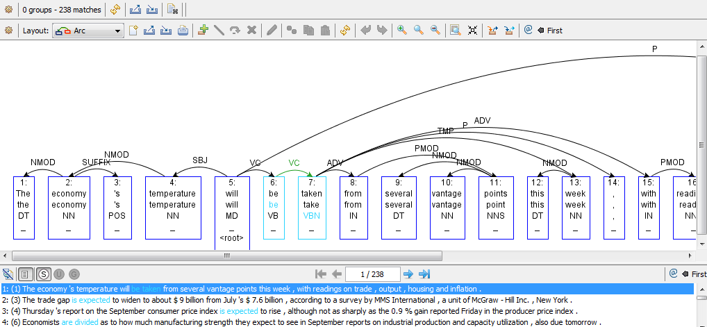
1. One grouping operator  used.
used.
Query:

Text Query: [lemma=be [relation=VC, lemma<*>1, pos=VBN]]
Result Toolbar:

All lemma types found are shown in the list (red) to the left. The user may select one lemma type to get all instances with matching query. Every occurence that matches the query is colored blue and the "grouped" lemma colored red. Results (1D) 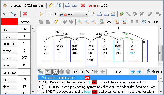
Options:

 = Switch between numeric/percentage result numbers (total)
  = Sort by wordform or by occurence (ascending/descending)
  = Reset list sorting
2. Two grouping operator  used.
used.
Query:

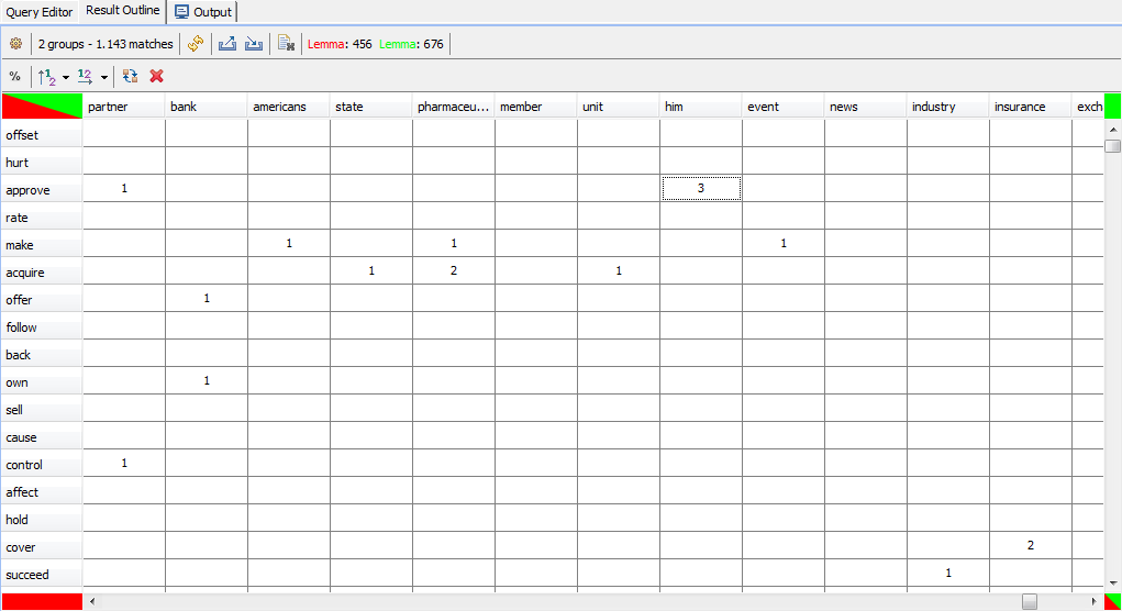
Text Query: [lemma=be [relation=VC, lemma<*>1, pos=VBN [relation=LGS, form=by [relation=PMOD, lemma<*>2]]]]
Result Toolbar:

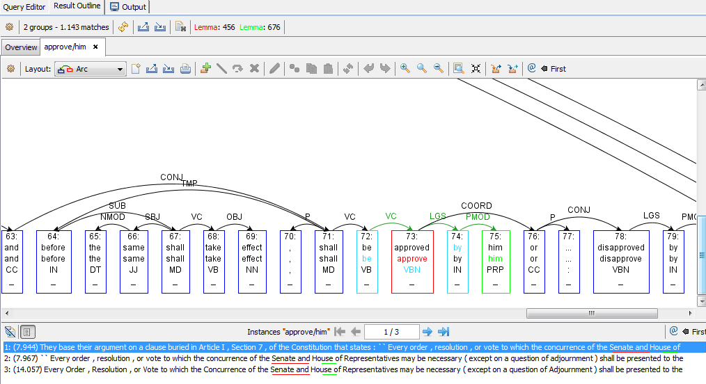
The result is presented as a table. Grouping operator one (red) is on the y-axis and grouping operator two (green) on the x-axis (Note: The x-/y-axis may be fliped clicking on  ). Every occurence that matches the query is colored blue. Results (2D)
Options:

 = Switch between numeric/percentage result numbers (total)
  = Sort y-axis by wordform or by occurence (ascending/descending)
  = Sort x-axis by wordform or by occurence (ascending/descending)
  = Swap the x-/y-axis (e.g.: (old) x-axis = (new) y-axis and vice versa)
  = Reset table sorting
3. Two grouping operator  used.
used.
Query:

Text Query: [lemma=be [relation=VC, lemma<*>1, pos=VBN [relation=LGS, form=by [relation=PMOD, lemma<*>2]][relation=OBJ, lemma<*>3]]]
Result Toolbar:

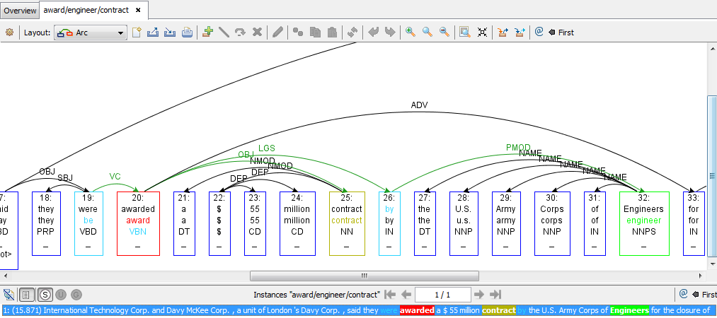
The result is presented as a list of sentences. Every occurence that matches the query is colored blue. Results (3D) 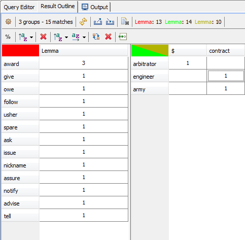
Options:

 = Switch between numeric/percentage result numbers (total)
  = Sort by wordform or by occurence (ascending/descending)
  = Reset list sorting
  = Sort y-axis by wordform or by occurence (ascending/descending)
  = Sort x-axis by wordform or by occurence (ascending/descending)
  = Swap the x-/y-axis (e.g.: (old) x-axis = (new) y-axis and vice versa)
  = Reset table sorting
  = Change the grouping operor ([0] = list, [1] = table y-axis and [2] = table x-axis). In this example
 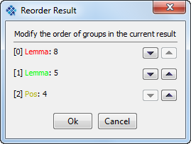 we have [0] = first
  (red), [1] = second
  (green) and [3] = third
  (brown)
1) Tutorial Dependency Search (passive constructions) with one grouping operator:
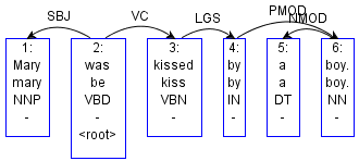
If the the user doesn't exactly know the how passive constructions are annotated in a treebank. Then he can use e.g. mate-tools or weblicht to parse a sentence contains a passice construction and copy&paste the structure to the search graph.
Parsed sentence "Mary was kissed by a boy."
 .
. Select the passice construction
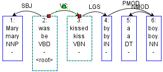
Copy the selected cells and edges
 and switch to the
Paste selected cells and edges into the search query editor window

The resulting graph when using the arc-layout (recommended)

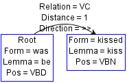
- In the following step the search graph (query) will be generalized (double clicking the edge / nodes to open the edge/node editor).
Node 1 properties
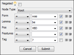 changed to
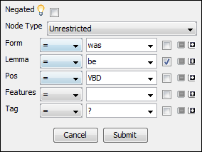
Edge properties
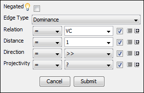 changed to
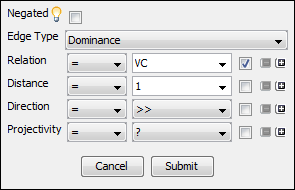
Node 2 properties
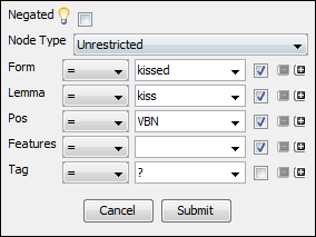 changed to (added grouping operator <*>)
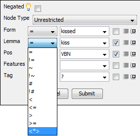
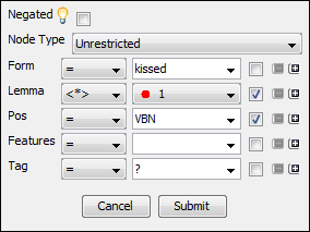
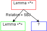
These changes result in a new more generalized version of the search graph (below is the textual query representation)
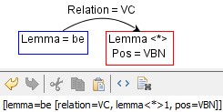 This query matches passive constructions in English as annotated in the CoNLL08 Shared Task data set.
2) Tutorial Dependency Search (passive constructions with overt logical subjects):
We are interested in passive constructions with overt logical subjects, grouped by lemma of the verb and the lemma of the logical subject. We may use the search graph for passive constructions or build the query completly manually (shown here).
First of all clear the graph editor panel (if there is any remaining graph) using

Add four new nodes
 you may "automatic reorder" them by clicking
Your graph editor should look like

- There are two ways connecting nodes / adding edges
Select two nodes
 and connect them clicking on
Place the cursor in the middle of the desired (source) node. A green border will show up
 . Hold the left mousebutton and move to the (target) node. When you reached the target node again a green border shows up. Release the left mousebutton to draw an edge between those node
Double click on the nodes/edges to specify the constraints. (Note: Adding constraints may mess up the graph layout. You may use
 to redraw the graph)
 Node 1: Lemma = be

Node 2: Lemma = <*> (red grouping operator); Part-Of-Speech = VBN

Node 3: Form = by

Node 4: Lemma = <*> (green grouping operator)

Edge 1: Relation = VC

Edge 2: Relation = LGS

Edge 3: Relation = PMOD

When every node, edge was linked and there was no error setting the constraints above the search graph should look like this:

(Textual query: [lemma=be [relation=VC, lemma<*>1, pos=VBN [relation=LGS, form=by [relation=PMOD, lemma<*>2]]]])
3) Tutorial Dependency Search (passive constructions with overt logical subjects and object):
In tutorial 1) we showed how to create a query using a copied graph from the parser. Tutorial 2) shows how to create a query from scratch. In tutorial 3) we will extend the search graph used in 2) with an additional grouping operator.
We start with the following search graph

Add one new node
 you may "automatic reorder" them by clicking
Your graph editor should look like

- Connect the "red" node with the new node using one of the following options
Select the node
 and connect them clicking on
Place the cursor in the middle of node 2. A green border will show up
 . Hold the left mousebutton and move to the new node. When you reached the target node again a green border shows up
  . Release the left mousebutton to draw an edge between those node
Double click on the new node/edge to specify the constraints. (Note: Adding constraints may mess up the graph layout. You may use
 to redraw the graph)
 Node 5: Lemma = <*> (browngrouping operator)

Edge 4: Relation = OBJ

When every node, edge was linked and there was no error setting the constraints above the search graph should look like this:

(Textual query: [lemma=be [relation=VC, lemma<*>1, pos=VBN [relation=LGS, form=by [relation=PMOD, lemma<*>2]][relation=OBJ, lemma<*>3]]])
