ICARUS-Search-Perspective
The  perspective provides the following search types:
- Dependency-Search
- Coreference-Documents
- Error Mining for Part-Of-Speech Tags
- Error Mining for Dependency Structure
Index:
I. How to set up a new search:
Click on
 to create a new search.
 - Afterwards the search need to be configured:

- Type: Select the desired search mode (dependency, error mining, coreference,...)
- Data-Set: Select the Treebank/Document
Query: Clicking
 opens the query editor. There may be different types of query editors depending on the search type.
 - Parameters: Search pararameters depending on the search type.
Execute Search using the
 button
 View the Result by double-clicking the search result or use the inspect-button

II. Search Menu:

 = Open the preferences
  = Create a new search
  = Executes the search. Note if no data-set was set the button is disabled
Search History Toolbar:  . Every executed search is listed in the search history. The history is available until you close your ICARUS session. The figure shows three search history items. During the search process the icons to the left may change:
 Search is active (first icon) but the target data-set is not loaded yet (second icon)
  Search is active (first icon) and target data-set is loaded (second icon)
  Search finished successful (first icon) and target data-set is loaded (second icon)
  Search was not successful.
  = Clear all search history items
  = Remove the selected search result from the history
  = Display the query of the selected search
  = Display the result of selected search
  Cancel selected search
III. Result Outline:
- Aggregated result visualization depending on the number of grouping operators (dimensions) for up to three groups (3D)
- Result highlighting for instances of query constraints
- Fully customizable graph visualization
- Easy navigation through results for up to three groups (3D)
IV. Dependency-Search
Search Parameter (Dependency-Search):
Search-Mode: Non-Exhaustive (stop after first hit), Exhaustive (add each sentence to the result at most one) and Exhaustive search with Grouping
Direction: Left-To-Right or Right-To-Left
Case-Sensitiv: On/Off
Result Limit: limit the search result (number of hits)
Graph Query Editor (Dependency-Search):
 This tab is used to build a query. Graph Editor Toolbar:
 = Open the preferences
  = Change the current graph layout. There are three different layout types available
Arc layout

No layout

Tree
 = Clear graph panel - every nodes/edges are deleted
  = Save the current search graph to XML file (may be imported later)
  = Import a search graph XML file
  = Print the current graph
  = Add a new node to the current search graph
  = Adds a new disjunction to the current search graph
  = Connects two nodes (two nodes must be selected before this action can be performed)
  = Connects two nodes with a precedence relation (two nodes must be selected before this action can be performed)
  = Delete selected node/edge (multi selection possible)
  = Opens the edit node/edge dialog (Instead of using this button you may doubleclick a node/edge to open the edit dialog)
  = Duplicate (copy and insert) the selected nodes/edges. Quick way to duplicate a graph. Note: edges are only copied when their source and target node is selected.
  = Copy and the selected nodes/edges. Note: edges are only copied when their source and target node is selected. (strg+c)
  = Paste previously copied nodes/edges. (strg+p)
  = Redraw the graph, can be useful while adding new nodes, edges or constraints may mess up the graph layout. Example (arc-layout): (left nodes/edges unsorted; right nodes/edges reorderes)
Note: The copy&paste nodes/edges can be used to copy graphs from/into other perspectives (e.g. Tutorial 1D,..)
 = Undo the last graph editor operation
  = Redo the last graph editor operation
  = Increase zoom level
  = Switch back to the default zoom level
  = Decrease zoom level
  = Autofit zoom level to the current graph panel size (default off)
  = Compress graph (right-left). Merge node/edge information into a node. Search annotation highlight is never merged and always visible even. (default off)
  = If there are different (unconnected) graphs A, B the search will use the following query (A v B).
Text Query Editor Toolbar: 
 = Undo the last text editor operation
  = Redo the last text editor operation
  = Copy and the selected text. (strg+c)
  = Paste previously copied text. (strg+p)
  = Select the entire query text (strg+a)
  = Clear the text query panel.
  = Save query graph to the current selected search history item
  = Generate search graph from text query
  = Generate text query from search graph
Result Outline (Dependency-Search):
 Use this tab to browse the search results. The visialization may be seperated into four differnet presentation styles. We describe the different types in the following section.
Result Outline Toolbar: 
 = Open the preferences
  Short query description and number of matches (here 3 grouping operators and 10 matches)
  = Refresh the result outline
  = Save the current search result to a XML file (may be imported later)
  = Import search result XML file
  = Close the result outline
  Grouping operator
  result informations. The corresponding
  color and the number of matches for each
  (ICARUS supports up to three grouping operators) (In this example we have 1. lemma-
  (red) 8 matches, 2. lemma-
  (green) 5 matches and 3. pos-
  4 matches)
0. No grouping operator  is used.
Query:

- Text Query: [lemma=be [relation=VC, pos=VBN]]
Result Toolbar:

The result is presented as a list of sentences. Every occurence that matches the query is colored blue. Results (0D) 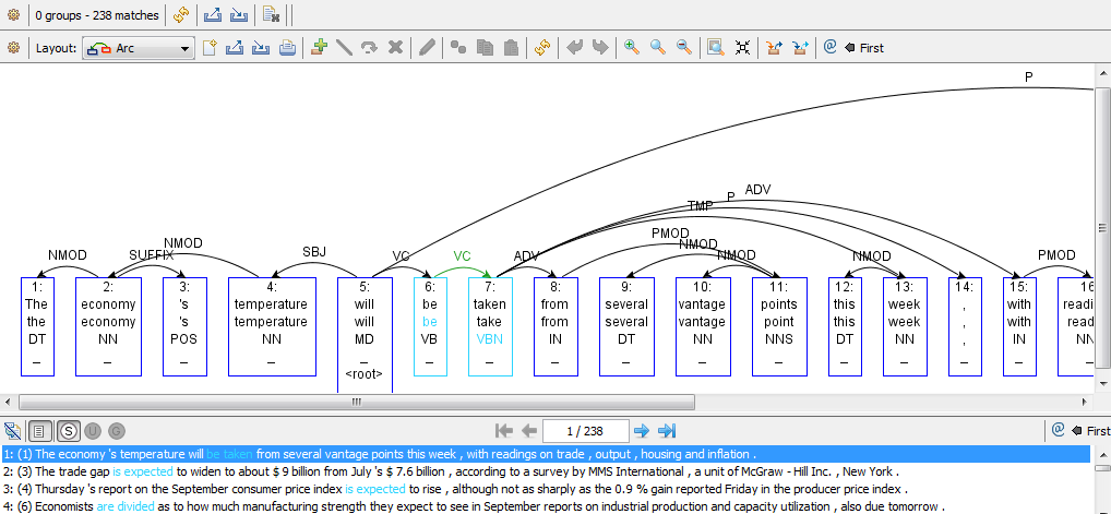
1. One grouping operator  is used.
Query:

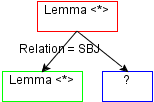
Text Query: [lemma=be [relation=VC, lemma<*>1, pos=VBN]]
Result Toolbar:

All lemma types found are shown in the list (red) to the left. The user may select one lemma type to get all instances with matching query. Every occurence that matches the query is colored blue and the "grouped" lemma colored red. Results (1D) 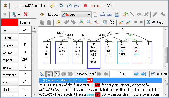
Options:

 = Switch between numeric/percentage result numbers (total)
  = Sort by wordform or by occurence (ascending/descending)
  = Reset list sorting
2. Two grouping operators  are used.
Query:

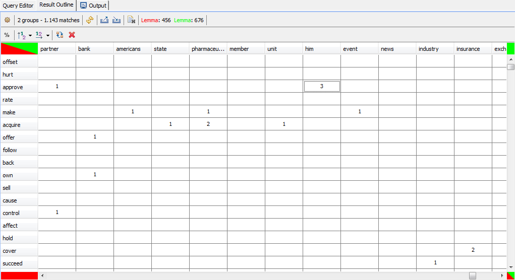
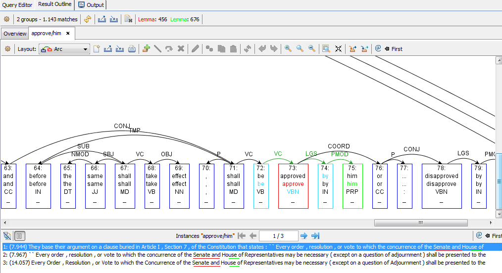
Text Query: [lemma=be [relation=VC, lemma<*>1, pos=VBN [relation=LGS, form=by [relation=PMOD, lemma<*>2]]]]
Result Toolbar:

The result is presented as a table. Grouping operator one (red) is on the y-axis and grouping operator two (green) on the x-axis (Note: The x-/y-axis may be fliped clicking on  ). Every occurence that matches the query is colored blue. Results (2D)
Options:

 = Switch between numeric/percentage result numbers (total)
  = Sort y-axis by wordform or by occurence (ascending/descending)
  = Sort x-axis by wordform or by occurence (ascending/descending)
  = Swap the x-/y-axis (e.g.: (old) x-axis = (new) y-axis and vice versa)
  = Reset table sorting
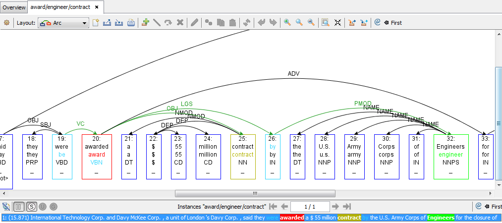
3. Three grouping operators  are used.
Query:

Text Query: [lemma=be [relation=VC, lemma<*>1, pos=VBN [relation=LGS, form=by [relation=PMOD, lemma<*>2]][relation=OBJ, lemma<*>3]]]
Result Toolbar:

The result is presented as a list of sentences. Every occurence that matches the query is colored blue. Results (3D) 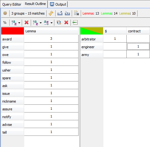
Options:

 = Switch between numeric/percentage result numbers (total)
  = Sort by wordform or by occurence (ascending/descending)
  = Reset list sorting
  = Sort y-axis by wordform or by occurence (ascending/descending)
  = Sort x-axis by wordform or by occurence (ascending/descending)
  = Swap the x-/y-axis (e.g.: (old) x-axis = (new) y-axis and vice versa)
  = Reset table sorting
  = Change the grouping operor ([0] = list, [1] = table y-axis and [2] = table x-axis). In this example
 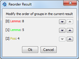 we have [0] = first
  (red), [1] = second
  (green) and [3] = third
  (brown)
At the lower part of the graph panel is the text outline. The list contains all search results of the selected instance. The selected sentence is shown in the graph panel.
Toolbar: 
 = Toggle a textpanel to copy the selected sentence. (see below)
  = First sentence
  = Previous sentence
  = Shows the current selected sentence (first number) and the total sentences (last number). In the example figure sentence 2 of 3 is selected. The user may navigate using the arrows to the left/right. It is possible to enter the sentence no. in this field by pressing "return" the sentence pops up. Note that the sentence numbers belong to the the internal index (the corpus index may differ for example if one sentence number have been skipped)
  = Next sentence
  = Last sentence
V. Error Mining
To detect sequence annotation errors within part-of-speech tags we implemented the algorithm introduced by Dickinson and Meurers (2003) [1]. Additionally for structured annotations we choose the approach shown in Boyd et al. (2008) [2] that targets inconsistency within dependency structures.
We designed and built a graphical user interface (GUI) that is easy to handle and user-friendly. Implementing state-of-the-art algorithms for error detection with an user-friendly interface increase the operation domain because the algorithms can be used by a wider audience without deeper knowledge of computers. It provides even non-expert users with the capability to find inconsistent pos tags and dependency structures within a corpus.
[1] Dickinson, M. and Meurers, W. D. (2003). Detecting errors in part-of-speech annotation. In Proceedings of the 10th Conference of the European Chapter of the Association for Computational Linguistics (EACL-03), pages 107–114, Budapest, Hungary.
[2] Boyd, A., Dickinson, M., and Meurers, D. (2008). On detecting errors in dependency treebanks. Research on Language and Computation, 6(2):113–137.
Search Parameter (Error Mining):
Replace all Numbers by Special Token: When the number wildcard replacement filter is enabled the algorithm checks for every word-form during the error mining process if the current word is a number. This is done using a regular expression that flags all words where the first letter is a number (0...9). These words will be replaced with a special NumberWildcard token. It provides the error mining algorithm with the capability to compare strings that contain different numbers and treat them equally in order to find variation within the non-number word-forms.
Use Fringe Heuristic: The fringe heuristic is used to filter n-grams where the nucleus occurs at the start/end of the n-gram. This is useful because when the nucleus is surrounded by words the probability that we find an error is higher.
Maximum NGram Size (passes): Limit the maximum n-gram size (size = algorithm iterations). By default this parameter is zero which is equivalent to ∞ .
Maximum Sentences for Input: The sentence limitation is used to limit the number of sentences that are used for the error mining. Starting at sentence one until the specified value x is reached. For example with a limit of 10,000 at most the first 10,000 sentences of the specified corpus will be used during the error mining process. Note: Using this option has a strong influence on the results and should be used carefully, because limiting the input data may leak the variation for one word. By default this value is "0" (zero) and the engine will use all sentences of the given corpus.
Show only NGrams with a size of: Even when the fringe heuristic is enabled the results will still contain uni-/bi-grams. Using the Show only NGrams with a size of option allows the user to filter the resulting n-grams. For example if the value is set to "1", the resulting list will contain 2-, 3-, n-grams, ... .
Create XML Output File: Using the Output to File option creates an xml-formatted file. It contains information about the word-forms, tags, tag-count and highlight information. It is formatted in a human-readable way so that its possible to do error detection even without the graphical support of the error mining plug-in. (By default no outputlocation is set in the
 and the user will be asked for the desired filelocation when the error mining task is complete)
Error Mining Query Editor:
 This tab is used to build a query. A single query item contain of the following parts:
Include Tag (boolean) = All tags that are ignored (Include Tag=true) are mapped onto a special "ignoredtag"-subclass. This option has priority over the new tag definition.
Tagclass (string) = If the current tag matches the Tagclass it may be included or assigned with a new Tag (if speficied)
new Tag (string) = The new tag for all tags that have a matching Tagclass within the query list specified in ii.)
If the current tag is not found within the query list it is neither ignored nor does it get a new tag assigned and the algorithm just continues the normal way taking the current tag. The benefit of this design is that there is no need to put the whole tag-set into the query system.
The Error Mining Query Editor provides the functionality to group tags together, rename tags or exclude tags from the search. It is organized in three parts 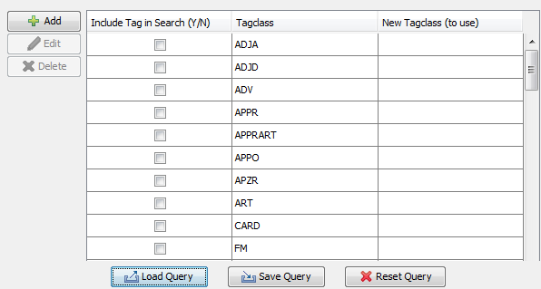 . On the left side there are buttons to create/edit or delete a single query:
In the middle there is an overview over all specified queries represented as a list. 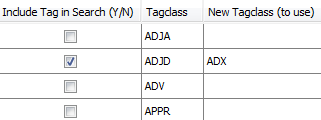
Below are three buttons to manage the ngram query item list:
 = Load ngram query xml file
  = Save all ngram query items to xml
  = Remove all ngram query items from list
The capability of saving a query to an extensible mark-up file (xml) and load it again later is useful if the user specifies a query and wants to use it later in different corpora. Using reset will delete all specified query items.
Result Outline(Error Mining):
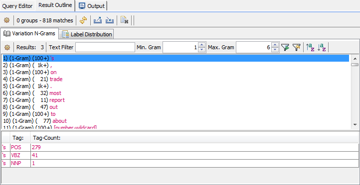
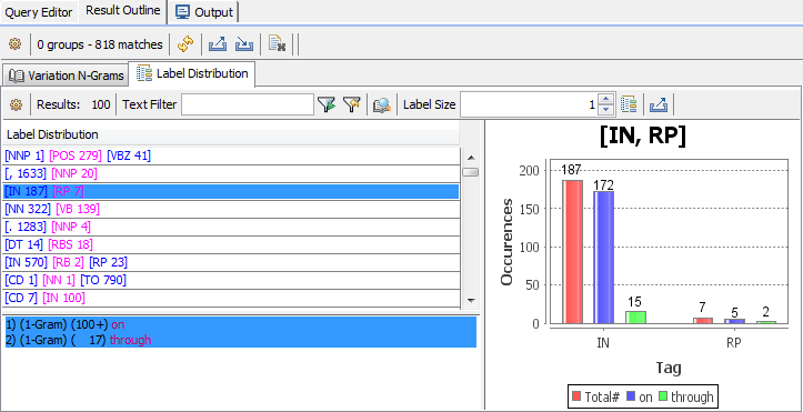
 Use this tab to browse the search error mining results. ICARUS provides two views for browsing the potential errors. The
  view shows a list of all variation n-grams found whereas the second view
  shows label distribution over word forms.
Result Outline Toolbar: 
 = Open the preferences
  Short query description and number of matches (note grouping is never used always "0" when viewing an error mining result)
  = Refresh the result outline
  = Save the current search result to a XML file (may be imported later)
  = Import search result XML file
  = Close the result outline
Variation N-Gram View (Error Mining):
Variation N-Gram Toolbar 
 = Open the preferences
  = Filter the variation n-gram list using the specified string
  = Minimum n-gram size for items within the list
  = Maximum n-gram size for items within the list
  = Apply variation n-gram filter
  = Reset variation n-gram list filter
  = Sort the n-gram ascending list by n-gram length
  = Sort the n-gram descending list by n-gram length
Each variation entry has the following format "Listindex) n-gram-length Occurence-Count ngram"
Example n-gram:  .
.
- "1)" List Index
- "1-gram" Length of the variation n-gram (here 1)
- "100+" Variation n-gram occurence count. (100+ = more than 100 matches)
- "'s" Every variation nucleus is colored purple
When the user selects one n-gram additional information about the nucleus (part-of-speech tags, tagcount) is displayed below the list. To inspect the result the user may double click on an entry from the variation n-gram lis. In the example he would recieve all sentences with the nucleus "'s" (POS, VBZ and NNP) clicking on 
If he is only interested in instances where "'s" was tagged as VBZ first he have to select the n-gram in the list and anfterwards double click on one of the lines in the lower part of the window  that contain that particular combination of word form and part-of-speech tag. Each time the user clicks on a n-gram, a new tab will be created, allows the user to jump back to previous results without having to recreate them (run the search again).
Label Distribution View (Error Mining):
Variation Label Distribution Toolbar 
 = Open the preferences
  = Filter the label distribution list using the specified string
  = Apply label distribution filter
  = Reset label distribution filter
  = Show sentences for the n-gram
  = Specify n-gram size for label distribution
  = Generate new label distribution for specified
  n-gram size
  = Export barchart to "portable network graphics" (.png) (export settings can be configured in the preferences
On the left a list of unique label combinations is shown. Selecting one displays a list of word form that occur with exactly these tags in the corpus. This list is below  . To the right the frequencies of the different labels are shown in a barchart. The left-most bar (here red) for each label always shows the total frequency. The user may select more words froms from the list to add additional bars to the chart that show the frequencies for eacht selected word form.
Results Presentation:
VI. Tutorials (including videos)
Tutorial Dependency Search (passive constructions) with one grouping operator
Tutorial Dependency Search (passive constructions with overt logical subjects)
Tutorial Dependency Search (passive constructions with overt logical subjects and object)
1) Tutorial Dependency Search (passive constructions) with one grouping operator:
Video Download:
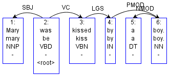
If the the user doesn't exactly know the how passive constructions are annotated in a treebank. Then he can use e.g. mate-tools or weblicht to parse a sentence contains a passice construction and copy&paste the structure to the search graph.
Parsed sentence "Mary was kissed by a boy."
 .
. Select the passice construction
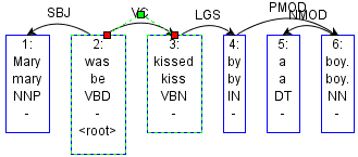
Copy the selected cells and edges
 and switch to the
Paste selected cells and edges into the search query editor window

The resulting graph when using the arc-layout (recommended)

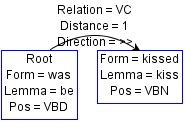
- In the following step the search graph (query) will be generalized (double clicking the edge / nodes to open the edge/node editor).
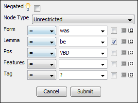
Node 1 properties
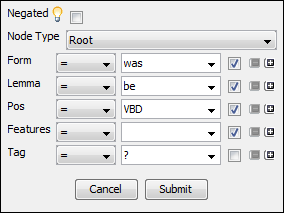 changed to
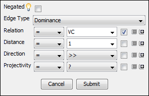
Edge properties
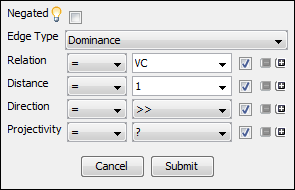 changed to
Node 2 properties
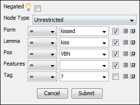 changed to (added grouping operator <*>)
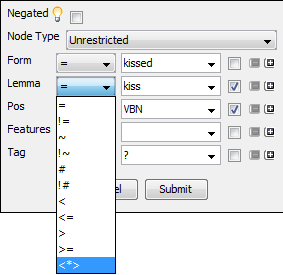
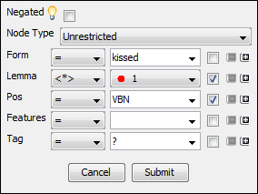
These changes result in a new more generalized version of the search graph (below is the textual query representation)
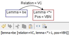 This query matches passive constructions in English as annotated in the CoNLL08 Shared Task data set.
2) Tutorial Dependency Search (passive constructions with overt logical subjects):
Video Download:
We are interested in passive constructions with overt logical subjects, grouped by lemma of the verb and the lemma of the logical subject. We may use the search graph for passive constructions or build the query completly manually (shown here).
First of all clear the graph editor panel (if there is any remaining graph) using

Add four new nodes
 you may "automatic reorder" them by clicking
Your graph editor should look like

- There are two ways connecting nodes / adding edges
Select two nodes
 and connect them clicking on
Place the cursor in the middle of the desired (source) node. A green border will show up
 . Hold the left mousebutton and move to the (target) node. When you reached the target node again a green border shows up. Release the left mousebutton to draw an edge between those node
Double click on the nodes/edges to specify the constraints. (Note: Adding constraints may mess up the graph layout. You may use
 to redraw the graph)
 Node 1: Lemma = be

Node 2: Lemma = <*> (red grouping operator); Part-Of-Speech = VBN

Node 3: Form = by

Node 4: Lemma = <*> (green grouping operator)

Edge 1: Relation = VC

Edge 2: Relation = LGS

Edge 3: Relation = PMOD

When every node, edge was linked and there was no error setting the constraints above the search graph should look like this:

(Textual query: [lemma=be [relation=VC, lemma<*>1, pos=VBN [relation=LGS, form=by [relation=PMOD, lemma<*>2]]]])
3) Tutorial Dependency Search (passive constructions with overt logical subjects and object):
Video Download:
In tutorial 1) we showed how to create a query using a copied graph from the parser. Tutorial 2) shows how to create a query from scratch. In tutorial 3) we will extend the search graph used in 2) with an additional grouping operator.
We start with the following search graph

Add one new node
 you may "automatic reorder" them by clicking
Your graph editor should look like

- Connect the "red" node with the new node using one of the following options
Select the node
 and connect them clicking on
Place the cursor in the middle of node 2. A green border will show up
 . Hold the left mousebutton and move to the new node. When you reached the target node again a green border shows up
  . Release the left mousebutton to draw an edge between those node
Double click on the new node/edge to specify the constraints. (Note: Adding constraints may mess up the graph layout. You may use
 to redraw the graph)
 Node 5: Lemma = <*> (browngrouping operator)

Edge 4: Relation = OBJ

When every node, edge was linked and there was no error setting the constraints above the search graph should look like this:

(Textual query: [lemma=be [relation=VC, lemma<*>1, pos=VBN [relation=LGS, form=by [relation=PMOD, lemma<*>2]][relation=OBJ, lemma<*>3]]])
4) Tutorial Error Mining:
Video Download:



 = Add a new ngram query item
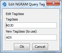
  = Edit selected ngram query item
 = Delete selected ngram query item